Geometric all-pass cascaded filter pairs

"Geometric" Filters

I'm not sure what to call the type of filter we've examined in previous posts, so let's just call them Geometric All-pass Pairs - or GAP filters. Because the world needs another acronym.

If you'll recall, we used a geometric mathematical sequence to arrange the poles and zeros in the complex plane, in order to produce some desired phase difference between a pair of filter cascades.

For the Hilbert transformer configuration, having -pi/2 phase difference (see previous posts),
the relevant generator equations which produce the appropriate pattern of poles and zeros can be written as:

      Filter A: exp(+/- pi*(2^-x))
      Filter B: exp(+/- pi*(2^-x) + i*pi)

      {x:0..n; n odd (equal to filter order, o-1)}
      [- for the poles; + for the zeros]

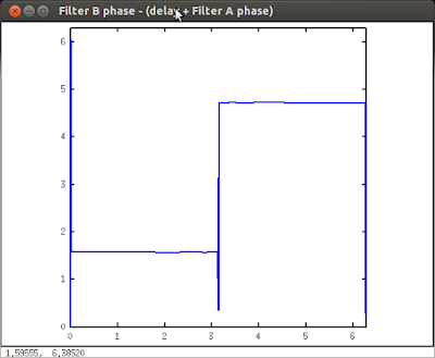
Figure 1 shows a plot of the phase difference of the Hilbert configuration:

A closer look at the pi/2 phase mark reveals that the response is not flat - we see a distinct ripple in-band, with a larger oscillation at either side of the pi/2 frequency:

Tweaking the phase response

It so happens that we can adjust the characteristics of the ripple by varying the significand in our generator function. For example, let's increase pi to 4 and re-examine the phase plot close-in.

The equations become:

      Filter A: exp(+/- 4*(2^-x))
      Filter B: exp(+/- 4*(2^-x) + i*pi)

And the plot now looks like:

Notice how the limits of the ripple are now confined to a tighter range.

We can further improve matters by this time changing the base of the generator function.
Let's reset the significand to pi and decrease the base from 2 to pi/2:

      Filter A: exp(+/- pi*(0.5*pi^-x))
      Filter B: exp(+/- pi*(0.5*pi^-x) + i*pi)

Again the close-up:

Now you can see we have a completely smooth response curve. However, as usual in signal processing, there is a trade-off: the effective bandwidth of the Hilbert transformer has been somewhat reduced.

We can reverse this bandwidth constriction by increasing the number of terms in the generator function:

Now the response is almost flat! But of course the trade-off has only been shifted elsewhere as we now need more sections to create the filter.

Second Order Coefficients

Talking of filter sections, we commonly construct filter banks using second-order sections (SoS) or 'biquads' (A biquad has a maximum of 2 poles and 2 zeros). Until now we have been thinking in terms of basic first-order pole and zero coefficients. What we'd like is a way to generate second order coefficients, which will make it more efficient to construct the filter with standard biquad building blocks. 

Fortunately, due to the quadratic nature of biquads (whence the name), this is just a matter of mutiplying out one real or conjugate pole-pair and one real or conjugate zero-pair for each SoS.

Our Hilbert configuration has only real poles and zeros, and it can be shown the biquad coefficient generator equation corresponding to the first-order pole/zero generator is:

   Filter B: exp(-2*significand*((base)^-(2*x)))
   Filter A: exp(-2*significand*((base)^-(2*x+1)))

   {x:0..m; m=(n-1)/2 }

[We have also made the equation more generic.]

This gives the Feed-Forward z-0 or 'ff0' biquad coefficients, which is all we need because,
as luck would have it, all of the z-1 (ff1) and z-2 (ff2) coefficients can be set to 0 and 1
respectively.

So, using our example of base=2 and significand=4 from figure 3, we get the biquad

numerator (feed-forward) coefficients:

(filter cascade A: order o=18; n=17; m=9)

   ff0       ff1       ff2
   ===========================
  -0.01832   0.00000   1.00000
  -0.36788   0.00000   1.00000
  -0.77880   0.00000   1.00000
  -0.93941   0.00000   1.00000
  -0.98450   0.00000   1.00000
  -0.99610   0.00000   1.00000
  -0.99902   0.00000   1.00000
  -0.99976   0.00000   1.00000
  -0.99994   0.00000   1.00000


(filter cascade B: order o=18; n=17; m=9)

   ff0       ff1       ff2
   ===========================
  -0.00034   0.00000   1.00000
  -0.13534   0.00000   1.00000
  -0.60653   0.00000   1.00000
  -0.88250   0.00000   1.00000
  -0.96923   0.00000   1.00000
  -0.99222   0.00000   1.00000
  -0.99805   0.00000   1.00000
  -0.99951   0.00000   1.00000
  -0.99988   0.00000   1.00000

Now apply the standard all-pass trick of reversing the feed-forward coefficient in order to get the feedback coefficients:

fb0(n) = ff2(n); fb1(n) = ff1(b); fb2(n) = ff0(n)

And remember we need a unit-delay in series with filter B. This can also be implemented with a biquad all-pass section (with reversed fb coefficients as above):

   ff0       ff1       ff2
   ===========================
   0         1         1

Simply add the delay biquad in series with filter B, and voila! an IIR Hilbert Transformer.

Conclusion

In this post we discovered a mathematical formula for the generation of coefficients for Hilbert transformers of arbitrary filter order, trading acceptable in-band ripple against maximum effective bandwidth.


The next time we will learn how to generate the biquad coefficients for the low-pass and high-pass filters which we previously obtained from the basic Hilbert configuration (see the post entitled "Transforming the Transformer" for the necessary background.)

RAW~

Transforming the Transformer

transforming the transformer

In the last post, Design of an all-pass Hilbert Transformer filter, we began with the pole/zero pattern shown in Figure 1:

Figure 1 - Hilbert Configuration in the s-plane

We then followed the process:

1. Divided the filter into 2 halves called filter A and B
2. Transformed into the z-plane
3. Added a unit delay in series with filter A

Which gave us a Hilbert Transformer - a filter bank that takes an input and produces 2 related outputs with phase difference 90°. You should read that post to remind yourself how the filter was divided into two - by interleaved poles and zeros (and not by the 2 lines shown on the s-plane)


There is an additional step in the above sequence that we can perform:

0. Transform in the s-plane

pole/zero translations

For example, figure 2 shows a shift or translation of -pi/2:

Figure 2 - shifting the Hilbert configuration by pi/2

This results in a 90° rotation in the z-plane compared with the Hilbert Transformer:

Figure 3 - both (shifted) filters plotted in the z-plane (distant zeros at  +/- 23.14i and +/- 4.81i omitted)

I have plotted both filters together but they should be considered as separate interleaved filters.

We can then follow steps 1,2 and 3 of the process to produce a pair of all-pass sections with the following phase response:

Figure 4 - phase difference between filter B and delayed filter A

This new filter bank produces a pair of outputs 180° apart in the range 0 Hz to pi/2 Hz and 0° apart in the range pi/2 - pi Hz.

If you sum the outputs of the filter, the low frequencies (0 < f < pi/2) cancel out whilst the high frequencies (pi/2 < f < pi) reinforce each other. The result is a high-pass filter with a cut-off frequency at pi/2 Hz

On the other hand, if you take the difference of the filter outputs the frequencies combine in the inverse sense and you have a low-pass filter. So we get 2 filters for the price of 1 - a bargain.

[We can equally do the pole/zero translation directly in the z-plane just by rotating the Hilbert configuration through 90° to take it from the real axis to the imaginary axis.]

transforming the transformation

There are additional geometric manipulations we can perform in the s-plane (or indeed the z-plane) to alter the transition frequency of the phase response of figure 4.

pole/zero scaling

We can break the pi separation of the two s-plane rows by squeezing them together (or moving them apart). 

Figure 5 - Hilbert shifted by pi/2 and squeezed by pi/2

This "pi/2 X pi/2" operation results in the z-plane distribution:

Figure 6 - the pair of interleaved (shifted and squeezed) filters mapped into the z-plane
(distant zeros at 16.36 +- 16.36i omitted for clarity)

Again, we follow steps 1,2 and 3 of the process to give the phase relationship:

Figure 7 - adjusted phase difference between filter B and delayed filter A

This new relationship has produced another low/high pass filter pair with the transition frequency now at pi/4.

You can easily see that by applying different degrees of 'squeeze' or 'stretch' on the pair of s-plane lines we can change the transition frequency to whatever we like. The only caveat is that when the transition frequency moves close to 0 or pi, you have to reduce the order of the filter (i.e. use a lower 'n' in the filter generator function) due to the poles and zeros of the z-plane conjugate pairs interfering with one another.

RAW~

Design of an all-pass Hilbert Transformer filter

Here is a interesting arrangement of poles and zeros (shown in the s-plane):

Figure 1 - poles and zeros arranged according to power-of-2 multiples of pi:

One row at jω= 0 and another identical arrangement at jω = pi.

Note the mirror symmetry of the poles and zeros in the jω-axis - this is what an all-pass filter looks like in the s-plane.

It's hard to tell from the figure, but there are n=20 poles and 20 zeros at jω=0 at the points:

σ = +/- [pi, pi/2, pi/4, pi/8 ... pi/(2^20)]

(with the same again at jω=pi.)

Lets (not entirely arbitrarily) divide the filter into 2 parts given by alternate pole and zero positions across the σ-axis:

Figure 2 - filter B. Poles and zeros at positions given by pi*(2^-(2n))

Figure 3 - filter A. Poles and zeros at positions given by pi*(2^-(2n+1))

We can convert these analogue filters to digital ones by employing the matched z transform (see previous post): z <- exp(s) - i.e. we simply take the exponential of each pole and zero:

Figure 4 - Filter B transformed into the z-plane (zeros at +/- 23.14  not shown)

Figure 5 - Filter A transformed into the z-plane (zeros at +/- 4.81 not shown)

Filters A and B exhibit very similar phase responses (and flat amplitude responses since they are all-pass), but what is really interesting is the difference between those phase responses:

Figure 6 - Phase difference between filter B and filter A

It would be nice if we were able to flatten out those phase slopes to produce some manner of constant phase difference. It turns out that you can achieve this by adding a delay in series with one of the filters, as demonstrated in figure 7.

Figure 7 - Phase difference between filter B and delayed filter A

The preceding analysis implies that if we were to create a parallel filter bank with filter B in one path and Filter A in series with a unit delay (z-1) in the other, we would have a means to produce a constant phase difference of pi/2 over a wide band of frequencies between 0 and pi (Nyquist).

There are actually theoretical limits at exactly 0 and pi/2 but the more pole/zero pairs (produced by higher 'n' in the filter generator equation, exp(pi/2^n)), the wider the effective band. Unfortunately the process has a diminishing return which comes at the cost of filter settle time - since poles positioned ever closer to the unit circle result in filter 'ringing'.

The order n=20 example under discussion has an effective bandwidth all the way from 1 Hz to 22049 Hz at sampling rate 44100 Hz (i.e. with Nyquist frequency = 22050 Hz).

This type of filter is known, by employing a touch of artistic licence, as a Hilbert Transformer. Although (unlike a true Hilbert Transformer) it alters the phase of the input reference frequency, it does produce an analytic signal - a 'real' and 'imaginary' pair which are pi/2 degrees out-of-phase.

RAW~

Poles, Zeros and the Matched z-transform

poles and zeros

If you're familiar with filters then you probably know that the poles and zeros of a digital filter, shown in z-plane plots, represent the roots of the filter's transfer function, H(z). 

You may even know that the distance of those poles and zeros from the unit circle and the angle they make with the x-axis determine the filter's amplitude and phase characteristics - which pretty much completely specifies the filter's frequency response.

All of which implies that digital filters can be designed by simple pole and zero placement on the z-plane. And indeed they can - with similar arguments to be made for analogue filters in the s-plane.

s-plane

The s-plane is a representation of the Laplace Transform belonging to the domain of analogue filters. It can be related, or mapped, to the z-plane of digital filters in a number of different ways - most commonly via the so-called Bilinear Transform (which is a mathematical method of converting s-plane coordinates into z-plane coordinates).

So, if you have to hand some particular analogue filter design, you can convert it into a digital filter design by applying the appropriate transform. 

Figure 1 - Analogue Butterworth filter in the s-plane

Figure 2 - Filter mapped into the z-plane

These transformations are useful because analogue filters have been around for much longer than digital ones, so you can leverage existing designs in the extensive literature on the subject.

It is even possible consciously design new digital filters in the analogue domain with the express intention of later applying some transform into the z-domain. With the Bilinear Transform that can be a mathematically tedious process, but there is another type of transform which lends itself nicely to digital design in the analogue world: the matched z-transform.

matched z-transform

Whilst the Bilinear transform maps the entire negative s-plane to the inside of the z-plane unit circle and the entire positive s-plane to the outside of the z-plane unit circle, the matched z transform maps thin horizontal strips of height 2*pi from the s-plane to the z-plane, as illustrated in the following 2 figures (imagine both figures extending to infinity in both x and y directions).

Figure 3 - Infinitely wide strips of height 2*pi in the s-plane (3 shown).

The highlighted strip jw = -1pi .. 1pi is the primary domain.

Green areas (-sigma) map to the inside of the unit circle (stable poles).

Red areas (+sigma) map to the outside of the unit circle (unstable poles).

Other strips are aliases because they map into the same region as the primary.

Figure 4 - The s-plane strips mapped into the z-plane via the matched z transform.

The mapping is described by the notation z <- exp(s).

The line jω=0 (-pi .. pi) in the s-plane maps to the unit circle in the z-plane.

The mapping is invoked by taking the exponential of any s-plane coordinate to get it's corresponding z-plane coordinate. Not forgetting that this is a complex exponential and so, in general (using Euler's formula):

exp(s) = exp(x + iy) 
       = exp(x) * exp(jy)
       = exp(x) * (cos(y) + jsin(y))

For example, the point:

s = -0.22252 + 0.97493i 

maps to:

z = 0.44926 + 0.66254i

as demonstrated in the Butterworth configuration shown in figures 1 & 2.

We must ensure that any pole/zero designs we make in the s-plane fall within the central strip, or at least be aware that any falling outside the strip will be aliased back inside.

That 2*pi strip thickness is convenient because the unit circle in the z-plane is 2*pi radians around  - i.e. the same as the length of the s-plane y-axis section from which it is mapped under this particular transform. Therefore we avoid the (additional) distortions inherent in the Bilinear Transform method and the associated (albeit necessary) pre-warping calculations.

Of course this comes at the price of invoking the computationally expensive exponential function ... but here at the rawfilter blog we don't worry about such trivialities.

Most filters I make are designed in this way, so this post will hopefully give you some background on some of those to come in which I will demonstrate some useful (or at least educational) designs.

RAW~

Other IIR all-pass Hilbert Transforms on the net

A few months ago I came across a very old post on the Hilbert Transform by +Olli Niemitalo on his blog over at iki.fi/o. At the time I was learning about the transform by reading Katja Vetter's brilliant and highly original audio tutorials on www.katjaas.nl, and she made some reference to Olli's version being superior to the old circa-1982 hilbert~ patch that comes bundled with Pure Data (Olli's is indeed far superior).

So I went over and started reading Olli's blog.

In his Hilbert post he reveals a set of coefficients, discovered by genetic algorithm, for making a parallel all-pass 8th order filter Hilbert Transformer. And actually it's pretty good - I've made a Pd implementation which I still use. I named the patch ollibert~ (sorry).

Figure 1 - Olli's coefficients in Pd

Anyway, that's what got me interested in this whole thing. Olli found his coefficients using some clever recursive let-the-computer-find-the-answer-for-me method, but I wondered if there was a more mathematical way to do it - and that led me to my (admittedly expensive, although I think more accurate) hogbert~ solution. So-named because it's fat, at least for an IIR solution.

Well, once I had Olli's coefficients I could go ahead and do some measurements in Octave and Pure Data to check how good they really are (and to have some point of reference for hogbert~).

Here are the results of that analysis.

Figure 2 - phase difference between ollibert~ outlets

As you can see from figure 2, the phase response is pretty good across a wide band between 0 and pi Hz.

Using the xyscope in Pure Data we can see exactly how wide:

Figure 3 - ollibert~ at 20Hz is ~99% accurate

The phase response is still 100*(0.496/0.5) = 99.2% accurate at 20Hz. But from there it starts to deteriorate:

Figure 4 - ollibert~ at 10Hz: phase difference is now ~0.41 pi

It's a similar story up at the higher frequencies, near Nyquist at 22030Hz (at 44100Hz SR).

Let's see what happens if we transform these coefficients in order to convert the Hilbert Transform into a Pi Transform:

Figure 5 - ollibert~ in Pi formation with pi/2 transition

That looks like a pretty decent phase response as well - you could get a good pair of low/high pass filters from that.

Now let's try to alter the transition frequency:

Figure 6 - ollibert~ in Pi formation with pi/4 transition

Now we see, unfortunately, the near-perfect phase responses beginning to deteriorate.

So we can conclude that these filter coefficients are very good for a reasonably wide-band Hilbert Transform, especially given the relatively low-order of the filters. But this comes at the price of inflexibility under transformation in the complex plane - they are not mathematically perfect.

Introducing the xyscope

This is a short post about a type of measuring device patch I made in Pure Data (Pd) called an xyscope. It helps a lot when testing other Pd objects like Hilbert Transformers.

An xyscope is a tool for measuring phase relationships between pairs of input signals by representing the phase difference as geometric shapes, ranging from a perfect circle through a distorted circle all the way to a completely flat circle (i.e. a straight line). 

It's probably best to go ahead and demonstrate with some examples:

zero phase (in-phase)

Figure 1 - Inputs in phase

1. In figure 1, the wave generator outputs a cosine wave from it's left and right outputs. The phase difference is set to 0.
2. Both cosines are received by the xyscope which measures the phase difference (highlighted in orange) and graphs the relationship as a NE - SW straight line on the main display. 
3. The left generator output is displayed in the oscilloscope for reference.

pi/2 (quadrature phase)

Figure 2 - Quadrature phase (pi/2)

1. In figure 2, the wave generator outputs a cosine wave from it's left and right outputs. The phase difference this time is set to -pi/2, so the right output is actually a sine wave.
2. The xyscope measures the phase difference (highlighted in orange in units of pi) and graphs the quadrature relationship as a perfect circle on the main display.

pi  (out-of-phase)

Figure 3 - Inputs out-of-phase

1. In figure 3, the wave generator outputs a cosine wave from it's left and right outputs. The phase difference this time is set to -pi, so the right output is the inverted left output.
2. The xyscope measures the phase difference and graphs the inverted relationship as a NW - SE straight line on the main display.

pi/4 (and miscellaneous phases)

All other phase relationships generate a distorted circle on the xyscope. 

Here is pi/4 for illustration:

Figure 4 - pi/4 phase difference

1. In figure 4, the wave generator outputs a cosine wave from it's left and right outputs with phase difference pi/4.
2. The xyscope represents this difference as a distorted circle.

So that is an overview of the xyscope.  It works by plotting the input signals against each other sample-by-sample in the main display, and by taking the arcsine and doing some trig for the number box measurements.

Let me know in the comments if you want the scope patch - I'll upload it once I've fixed the last few bugs!

Phase splitters (part 2)

In the last post I promised to demonstrate some of the phase relationships obtainable from phase splitting parallel networks of all-pass filters - a technique known as polyphase IIR. So lets go ahead and do that. Here I will use GNU Octave to create the filters and produce the graphs.

Remember that all the phase plots in this post can be obtained from the same basic filter coefficients subjected to various transformations in the complex plane.

Hilbert Transform

The first plot demonstrates the classic Hilbert Transform configuration, which produces a phase difference of pi or 90 degrees. The 2 output signals are known as the reference signal and the quadrature signal.

Figure 1 - Phase relationship of the Hilbert Transform

The x-axis shows the frequency in radians (note the discontinuities at 0 and pi radians.)

The y-axis gives the phase difference of the 2 outputs: pi/2 from DC+d to Nyquist-d.

d is around 0.00014 radians in this order-20 set-up, which equates to 1Hz at 44100Hz SR.

The Pi Transformer - 2 filters for the price of 1

The second plot has a phase difference of pi in a slightly lower order (i.e. fewer poles and zeros) implementation of the same basic configuration.

Figure 2 - pi phase relationship

The outputs are exactly out-of-phase between DC (0) and 0.5*Nyquist (pi/2)

If the outputs are added we have a high-pass filter with cut-off frequency pi/2.

If the outputs are subtracted we have a low-pass filter with the same cut-off f.

We can combine the outputs with a simple addition or subtraction to produce a low pass or high pass filter, so we get 2 for the price of 1!

Variable transition frequencies

We can re-transform the transformed filter of figure 2 to produce different transition frequencies:

Figure 3 - pi phase relationship with different transition freq

The spike at pi/4 is due to phase-wrapping: a phase difference of 2*pi is

equivalent to a difference of 0 - i.e both imply exactly in-phase.

Series Combinations

If we combine the Hilbert transformer and Pi transformer in series we see the following phase relationship:

Figure 4 - Hilbert and Pi transformers in series

In this set-up filter output 2's phase lags output 1's phase by pi/2 all the way from 0 - pi/2  radians, at which point the relationship flips and output 2's phase leads output 1's phase by pi/2 radians.

Complex Filters

In this final graph you will see an example with a complex filter pair - whose complex coefficients do not come in conjugate pairs.

Figure 5 - Phase difference in complex filter network

The outputs of the complex filter array can be "decomplexified" (and therefore realized) by passing the each one through a special combination of none other than the Hilbert Transformer itself.

You're probably wondering about now just what are this set of filter coefficients that can produce so many types of filter? Don't worry - I'll get into those details in another post!

Phase Splitters (part 1)

I'm going spend my first few posts talking about a class of filter networks whose purpose is to transform an input signal into 2 (or more) output signals with some desired phase difference between them.

Normally such networks will take the form of a pair with output phase differences of:

1.  90° (π/2) known as a 'Hilbert Transformer' - although not strictly speaking a Hilbert transform because the input phase is not preserved.
   
2. 180° (π) which can be used as a low or high pass filter when the output pairs are combined

Other phase relationships are possible, especially if complex filters are used.

As you might expect when talking about phase (and not magnitude) filtering we are referring to networks of all-pass filters:

Figure 1 - All-pass phase-splitter network

Figure 1 shows the input signal(s) being phase-distorted by a pair of appropriately configured all-pass networks such that the phase of output 2 lags that of output 1 by π/2 (i.e. Hilbert Transform). The input phase may be (and probably will be) different to both.

It turns out that there is a particular set of filter coefficients which can serve as the basis for generating any number of pairs of all-pass sections with arbitrary phase split, accurate to an arbitrary bandwith (with theoretical limitiations at DC (0 Hz) and the Nyquist frequency (π Hz)). Furthermore, each section pair so-generated can be cascaded with other alternatively configured pairs to produce more complicated (yet predictable) phase relationships.

The set of generating filter coefficients are subjected to various transformations on the complex plane to produce the different classes of filter pair.

In the next post I will demonstrate some examples of phase difference relationships I created in back in my 'research labs' - i.e. sitting on the couch with an old laptop running GNU Octave and Pure Data (Pd).